 Ridvan Senturk, PMP
The situation
Article 001 ended with about 5,900 remaining labour hours on a synthetic 10,000-hour scope. Suppose that estimate is sound. Your forecast update is due — and the question you actually get asked is not how many hours are left. It is how many people, starting when.
The highest weekly average in the schedule is 50 worker-equivalents. You can field 30 qualified workers. The monthly report shows about 18 full-month equivalents.
In brief
This piece starts where Article 001 finished: with a credible estimate of remaining labour hours, and no crew plan. Hours on their own do not give you one — they need placing against the schedule, converting into a resource figure whose window and calendar are stated, and testing against the labour you can actually field and the workfront that is actually ready. On the way, the same hours produce several different figures, all arithmetically correct, none of them a headcount. Required demand and available capacity are different quantities, and resource levelling is the established practice for reconciling them. What I want to do is walk the chain end to end on one set of numbers that reconcile.
5,900 hours. How many people is that?
There is no answer to that question yet.
An estimate to complete is a current estimate of the resources still needed to finish the remaining scope.1 Here, ETC is expressed as remaining labour hours. That total alone does not tell you when the hours will be worked or how many people are needed at once. At 40 hours per person per week, 10 people for 15 weeks and 30 people for five weeks both provide 6,000 hours — roughly the effort in this example, with very different staffing patterns.
Here is the synthetic project I will use throughout. It is not drawn from any real job; the figures are chosen so the arithmetic reconciles and a reader can check it. One trade, unnamed. For this example, status is recorded through the end of Thursday 15 October 2026; remaining work starts Friday 16 October. Monday to Friday, eight hours a day, no holidays or overtime. Remaining quantities are unchanged since the last update.
From Article 001: a 10,000-hour budget, 5,000 hours earned, 6,250 hours spent, and a forward labour performance judgment of 0.85 — giving an estimate to complete of 5,882 hours (5,000 ÷ 0.85 = 5,882.35, carried as 5,882 in every calculation below; I will say “about 5,900” in prose). That 0.85 is Article 001’s assumed judgment for this scenario, not a measured rate, and how it was chosen is that article’s subject. Assume it is sound.
Now: how many people?
When does the schedule say you need them?
Placing those hours against the current schedule is what turns effort into a profile. Resource loading assigns the expected labour to scheduled activities so it can be analysed through time,2 and the output is the shape in Figure 1.
Figure 1
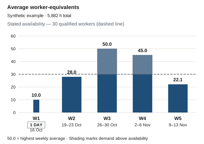
| Week | Working days | Hours | Average worker-equivalents |
|---|---|---|---|
| W1 · Fri 16 Oct (one-day partial week) | 1 | 80 | 10.0 |
| W2 · 19–23 Oct | 5 | 1,120 | 28.0 |
| W3 · 26–30 Oct | 5 | 2,000 | 50.0 |
| W4 · 2–6 Nov | 5 | 1,800 | 45.0 |
| W5 · 9–13 Nov | 5 | 882 | 22.1 |
| Total | 21 | 5,882 |
This is the first thing the chain adds, and it is why a total on its own cannot be staffed. It is also worth noticing what the profile does not yet tell you: whether 50 worker-equivalents can be found, and whether there is anywhere for them to work.
What does an FTE number actually tell you?
Before going further, a detour — because this is where the same hours start producing different numbers, and where a reader of a monthly report can end up with a figure that is correct and still the wrong one for the decision in front of them.
The same hours can produce different figures, each answering a different question. Three of those differences matter here, and they are separate problems.
First: the width of the bucket
Set the project aside for a moment. This is a standalone synthetic example with its own assumptions.
Neither figure is an error. Under the stated assumptions — four working days, eight hours per person per day — the activity averages 5 FTE across its execution window, and it also averages 1.0 FTE across a month that contains it. Both are true, and neither establishes a daily roster.
But if the question is what does this activity need while it is running, the monthly figure is not the one to read. A wider reporting bucket can average a short-duration requirement across time and make the execution intensity look much smaller than it is.
The settings matter as much as the timescale. In P6’s Resource Usage Profile, Calculate Average can use a manually entered divisor. With Base on Hours Per Timeperiod selected, it uses the corresponding User Preferences conversion. Check the divisor as well as the timescale.3 Oracle’s cloud resource planning likewise defines FTE over a specified planning interval and permits fractional values.4
The micro-example uses a 20-day month; October 2026 has 22 weekdays.
Second: matching the window to the hours
Back to the project. Suppose 3,200 of the 5,882 remaining hours fall in what is left of October — that is W1, W2 and W3 in Figure 1, and it is a defined subset of the estimate, not a second total.
Status runs through the end of 15 October. October 2026 has 22 weekdays; 11 of them fall after the 15th.5
| Question being asked | Hours | Working days | Denominator | Result | Correct label |
|---|---|---|---|---|---|
| How much October effort remains, in full-month terms? | 3,200 | 22 | 176 h | 18.18 | full-month equivalents |
| What is the average demand over the remaining October window? | 3,200 | 11 | 88 h | 36.36 | average worker-equivalents, 16–31 October |
| Alternative cutoff: if the same 3,200 h remained at the start of 15 October | 3,200 | 12 | 96 h | 33.33 | average worker-equivalents, 15–31 October |
| What is the average demand in the busiest week? | 2,000 of the 3,200 | 5 | 40 h | 50 | 50 average worker-equivalents, 26–30 October |
36.36 is twice 18.18 because the remaining-window denominator, 88 hours, is half the full-month denominator, 176 hours. Neither result is wrong. Calling 18.18 the average demand over the remaining eleven days would be misleading — but calling it 18.18 full-month equivalents of remaining effort is mathematically valid, just less useful for that particular decision. The problem is the combination of numerator, denominator, window and label, not the act of dividing by 176.
The third row is a comparison convention, not additional work in the main schedule: it shows what the same 3,200 hours would give under a start-of-day cutoff instead of an end-of-day one.
Third: an average is not a daily requirement
Here is the part that connects back to Figure 1.
The remaining October window averages about 36 worker-equivalents; its busiest week averages 50. Neither figure identifies the daily peak.
Both describe the same 3,200 hours. The window average is right and it is still not the number you staff to, because an average across a window says nothing about the distribution inside it. Nor is 36.36 thirty-six physical people: the total alone gives a lower bound of 37 full-time workers over the remaining window. That would not meet this profile’s 50-equivalent week without moving work; daily and skill requirements still need checking.
So the sequence runs: hours → stated window → average demand → check daily demand and readiness → crew decision. Each step answers something the previous one could not.
The schedule wants 50. You can field 30.
Now the two quantities meet.
Figure 1’s highest weekly average is a conditional demand result — what the schedule requires, given its current dates, logic and resource assignments. The 30 is a stated availability assumption — the qualified labour taken to be fieldable, over a matching calendar and interval. They are different kinds of number and it is worth keeping them apart. One is implied by a plan; the other is a stated assumption about what can be supplied.
The comparison only means anything when the intervals, qualifications and calendar match. If one figure is weekly and the other monthly, first express both over the same interval. On matched terms, this profile shows a shortfall of 20 worker-equivalents in the week of 26 October, and a smaller one the week after.
Two things are worth saying plainly, because both are tempting and both are wrong.
Reporting 50 as if it were an achievable staffing commitment, without addressing the difference, is unsupported by anything. And reporting only 30, without the work and dates it affects, is incomplete for a decision about resources versus dates. A gap on its own does not produce a feasible plan either.
What resource levelling actually does
None of this is a discovery. Reconciling required resources against limits is what resource levelling is for, and it has been for a long time.
Levelling can resolve modelled resource conflicts by changing timing or assignments. Usable float in the affected activities may absorb the change; where it does not, the finish may move. Recognised guidance treats this explicitly as a resource-versus-time trade-off, and the scheduling standard describes resource limits, priorities and date recalculation, with stakeholder review of the result.7 It is also worth knowing what the standard warns against: manipulating logic or date constraints to force a preferred histogram is not a substitute for levelling.7
Here is a simplified weekly capacity illustration, not a software-generated CPM result. Assume work cannot be brought forward into earlier weeks, excess hours can move into later weeks, and those later workfronts are available. Keep total hours unchanged and limit each full week to 30 × 40 = 1,200 hours.
Figure 2
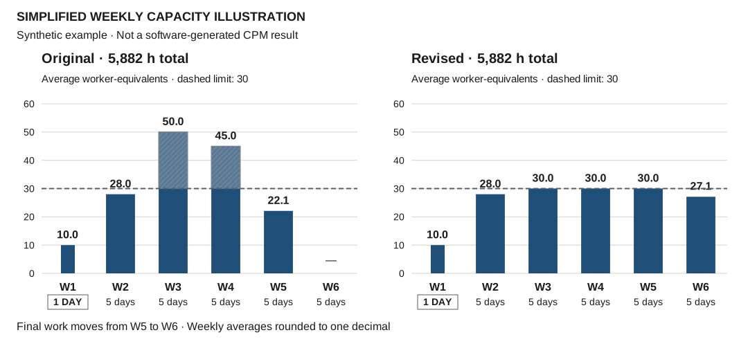
| Week | Working days | Original hours | Original average | Revised hours | Revised average |
|---|---|---|---|---|---|
| W1 · Fri 16 Oct (one day) | 1 | 80 | 10.0 | 80 | 10.0 |
| W2 · 19–23 Oct | 5 | 1,120 | 28.0 | 1,120 | 28.0 |
| W3 · 26–30 Oct | 5 | 2,000 | 50.0 | 1,200 | 30.0 |
| W4 · 2–6 Nov | 5 | 1,800 | 45.0 | 1,200 | 30.0 |
| W5 · 9–13 Nov | 5 | 882 | 22.1 | 1,200 | 30.0 |
| W6 · 16–20 Nov | 5 | — (no work in the original profile) | — | 1,082 | 27.1 |
| Total | 5,882 | 5,882 |
Read the two totals. They are identical. The illustration did not change how much work there is; it changed which week the work sits in, and here the last work moves into the following reporting week.
One bookkeeping point worth keeping straight: the 3,200 October hours used in Table 1 belong to the original demand profile. After this redistribution, October carries 2,400 hours. The FTE demonstration above is not the capacity-adjusted October forecast.
What a levelling calculation does not do is authorise anything. It calculates within the limits it has been given. It does not establish that every real workfront, qualification or release condition has been modelled, it does not decide whether to go and find twenty more people, and it does not choose a contractual date. Those are management decisions, and the calculation informs them rather than making them.
The honest general answer on what to send is: report a clearly labelled current plan, consistent with the resource assumptions you actually adopted. Where additional resources or date changes are still undecided, retain the conditional demand, the availability difference and the alternatives that decision needs. Do not silently treat demand as a commitment, or a levelled curve as proof of readiness.
That is a synthesis of the evidence and the decision logic — not a rule requiring two histograms on every update. P6 can preserve scheduled early and late dates during levelling. Separately, Oracle’s portfolio resource planning can show demand and allocation. Neither capability by itself establishes that a complete original demand histogram survives a CPM levelling run.8
Is the work actually ready?
A levelled plan says the resource limit has been respected. It does not say there is anywhere to work.
Readiness lives at a different planning level, and that is by design. Milestone and pull planning, make-ready, weekly commitments and learning are distinct conversations, and different detail at different horizons is deliberate rather than a defect.9 A master schedule need not carry every room-level readiness detail. A linked lookahead can hold that detail, with material consequences reflected in the forecast.
So take the familiar case. A master activity — Install X, Area A — covers four rooms. Room 101 is constrained; 102, 103 and 104 are ready.
Figure 3
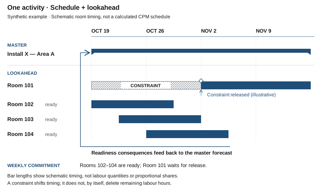
Two failure modes sit either side of the useful answer. Suspending the whole activity could conceal independently workable rooms. Leaving the access restriction unrepresented anywhere could conceal the problem.
There is a third option. The activity can carry a lower rate of labour through the currently available workfront, with the blocked work shifted into a later window. The total remaining hours do not disappear simply because part of the workfront is unavailable.
That distinction matters more than it looks. A blocked workfront does not, by itself, justify reducing the remaining labour. The work still has to be done; what has changed is when it can be done. Reducing the hours because a room is shut would be an estimating change, and it would need its own basis — not an access restriction. Nor do three ready rooms establish 75% of the remaining work, labour capacity or usable workfront.
Which leaves the useful question. Not should the master schedule contain rooms? — but does Room 101’s status reach the forecast? Several answers are possible and the example alone does not decide between them. If room readiness is reliably linked and rolled up, the aggregation may be entirely appropriate. If the whole activity has been suspended while three rooms are independently workable, that looks like an activity-design or status-treatment issue. If the rooms are shown ready but prerequisites are missing, it is a make-ready verification problem. And if a field change alters a milestone or resource consequence while the master forecast stays unchanged, that is a reconciliation problem.
Related readiness and information-flow failures are documented in an early Last Planner pilot, where deficiencies in readiness and information supply were recorded.10 That is evidence the failure mode exists — in a bounded case, decades ago, not a statement about how often it happens now.
The practical test is simpler than the taxonomy: feed material milestone or resource consequences back into the forecast; the two plans need not contain identical detail.
Same hours, different dates
Look again at Table 2. The last work moved into the following week and the total stayed at 5,882 hours. A change in dates does not, by itself, change how much labour remains.
P6 allows future-period remaining units to be updated without changing the original plan.11 That capability does not make effort and timing independent on a real project.
And here is the condition. Unchanged work content and unchanged effort assumptions permit rescheduling without changing the total. Overtime, remobilisation, congestion, resequencing or other productivity changes can alter ETC; each needs its own estimating basis.12 If you believe a delay will cost hours, that is a new estimate, and it needs its own basis.
The practical version: when something slips, ask which you are changing — the hours, the dates, or both — and record which one you touched.
When the forecast changes, what should be visible?
If the crew profile someone is staffing to has materially changed, the change is worth being able to explain.
There is a distinction here that is easy to blur. Issuing or approving a current forecast is not the same act as changing an approved baseline or budget. They are different objects with different purposes — and both exist. Recognised guidance calls for status changes to be documented, salient changes justified, and the current schedule version archived after management approval.6 DOE’s 2016 EVMS guidance provides for revised estimates at completion submitted for project-manager approval,13 and a scheduling recommended practice recognises acceptance and approval of schedule updates.14 So forecast approval is a real thing in real governance, not a category error.
Approval does not establish forecast accuracy or, by itself, authorise expenditure.
Who decides is genuinely local. The scheduling standard involves the team and key stakeholders; the EVMS guidance assigns forecast responsibilities to control-account managers and the project manager, with functional management involved where there are resource shortages; a scheduling practice distinguishes contractor preparation from owner or reviewer acceptance.71314 Preparation authority, the authority to commit crews, and the authority to move a milestone can sit with three different people. A scheduler’s calculation authorises none of them. The sources reviewed here do not prescribe one universal field-signature or forecast-owner arrangement.
The ways of resolving a resource shortfall — sustained overtime, adding crew quickly, compressing into a shorter window, resequencing — are among the conditions Article 001 asked us to review before setting a forward labour performance assumption. So the fix at the end of this chain can bear on the assumption at the beginning of it. That is an inference rather than a measurement, and I am not going to quantify it here.
Key takeaways
- Remaining labour hours answer how much effort is left. That total alone does not answer how many people, starting when — that needs the schedule, a calendar and a stated window.
- The same hours produce different, individually correct resource figures depending on the interval used, and a wider reporting bucket can average a short-duration requirement into something that looks much smaller.
- No resource equivalent is a headcount. The remaining October window averages about 36 worker-equivalents; its busiest week averages 50. Neither figure identifies the daily peak.
- Resource levelling reconciles modelled demand with resource limits. In this example it moves hours between weeks without changing the total; changed effort assumptions would require an ETC revision.
- A blocked workfront changes when work can be done. Reducing the hours would be an estimating change and needs its own basis.
Open questions
I would value practitioners’ experience on any of these.
- At a mid-month data date, what window does your manpower report actually use — and does its label say so?
- When demand exceeds the crew you can field, what do you publish: the requirement, the resource-limited plan, or both? Does the person reading it know which they have?
- When a room or area is not ready, where does that fact live — and does it reach the labour forecast, or stop at the lookahead?
- In your general practice, what does “approved forecast” mean: an issued version, a commitment, budget authority, or something else?
References
-
AACE International. Recommended Practice 10S-90: Cost Engineering Terminology — “Estimate to Complete.” https://web.aacei.org/docs/default-source/rps/10s-90.pdf?sfvrsn=20 ↩
-
U.S. Government Accountability Office (2015). GAO Schedule Assessment Guide: Best Practices for Project Schedules, GAO-16-89G — resource loading as allocating expected labour to scheduled activities and analysing them through time. https://www.gao.gov/assets/680/674404.pdf ↩
-
Oracle. Primavera P6 Professional Help, Version 24 — Define the Resource Usage Profile: Regular Histogram, step 10 (“Calculate Average”, “Divide Interval Totals By”, “Base on Hours Per Timeperiod”); page last published 4 March 2025, accessed 8 September 2026. Vendor documentation, cited for capability only. The 8-hour day and 40-hour week appear there as User Preferences examples, not universal calendar settings. https://docs.oracle.com/cd/F88968_01/client_help/en_US/define_the_resource_usage_profile_-_regular_histogram.htm ↩
-
Oracle. Resource Planning Overview — Understanding Role Availability. Vendor documentation, cited for capability only; establishes period FTE with fractional values as a product convention, not a construction staffing standard. https://docs.oracle.com/cd/E80480_01/help/en/user/109148.htm ↩
-
Calendar computation for October 2026: 22 weekdays; 11 after 15 October (16, 19–23, 26–30); 12 including the 15th. Assumes Monday–Friday, 8 h/day, no holidays or overtime — a synthetic assumption, not a claim about any actual local work calendar. ↩
-
GAO (2015). GAO Schedule Assessment Guide, Best Practice 9, printed pp. 129–130 — separation of actual and future status at the status date; documentation of status changes, justification of salient changes, and archiving of the current schedule after management approval. https://www.gao.gov/assets/680/674404.pdf ↩ ↩2
-
GAO (2015). GAO Schedule Assessment Guide, Best Practice 3, printed pp. 57–61 — resource levelling as a resource/time trade-off; and PMI (2011). Practice Standard for Scheduling, 2nd ed., printed p. 32 and resource levelling p. 69 — resource limits, priorities and date recalculation with stakeholder review, and a caution against manipulating logic or date constraints as a substitute for levelling. These describe the technical discipline, not an automatic choice of management action. https://www.gao.gov/assets/680/674404.pdf · https://www.pmi.org/-/media/pmi/documents/public/pdf/certifications/practice-standard-scheduling.pdf ↩ ↩2 ↩3
-
Oracle P6, preserve-dates and within-float levelling options; and Oracle, Specify Role Demand, separate demand and allocation views in portfolio resource planning. Vendor capability only. The first does not promise preservation of a complete original demand histogram, and the second is portfolio resource planning rather than a levelled CPM schedule. Neither demonstrates reporting effectiveness. https://docs.oracle.com/cd/F74773_01/p6help/en/91573.htm · https://primavera.oraclecloud.com/help/en/user/102271.htm ↩
-
Lean Construction Institute. Last Planner System — milestone and pull planning, make-ready, weekly promises and learning as distinct conversations at different horizons. https://leanconstruction.org/lean-topics/last-planner-system/ ↩
-
Ballard, G. (1997). Lookahead Planning: The Missing Link in Production Control, printed pp. 13, 24–25. A bounded pilot documenting deficiencies in readiness and information supply; evidence that the phenomenon exists, not evidence of its present-day prevalence. https://www.iglc.net/Papers/Details/17/pdf ↩
-
Oracle. Primavera P6 Professional User Guide — Future period bucket planning, 29 May 2026, update-remaining-units paragraph. Vendor documentation, capability only; separate editability is a software fact and does not make effort and timing independent on a real project. https://docs.oracle.com/cd/G48902_01/English/User_Guides/p6_pro_user/future_period_bucket_planning.htm ↩
-
Inference, not a standard: unchanged work content and effort assumptions permit rescheduling without changing total remaining hours, while overtime, remobilisation, congestion, resequencing or other productivity changes would each require a separate estimating basis. ↩
-
U.S. Department of Energy (2016). Earned Value Management System Interpretation Handbook, v2.0, printed pp. 113–115, Guideline 27.A.1–3 — revised control-account estimates at completion submitted for project-manager approval, with resource and schedule reconciliation. An EVMS example, not a universal construction rule and not a statement of current contractual requirements. https://www.energy.gov/sites/prod/files/2016/08/f33/DOE%20EVMSIH%20V2%200_08302016_FINAL.pdf ↩ ↩2
-
AACE International (2008). Recommended Practice 53R-06, rev. 14 August 2008 — sample printed page 1, recognising acceptance and approval of schedule status updates. Guidance rather than a standard by its own statement of purpose; the full practice was not inspected. https://web.aacei.org/docs/default-source/toc/toc_53r-06.pdf ↩ ↩2